Calculation and application of the Species Synanthropy Index: tutorial
Loïs Morel1
Nadege Belouard2
Baptiste Bongibault
Gurvan Le Floch
2026-04-21
01_SSI_SCI_Brittany.RmdThe SynAnthrop package computes a Species Synanthropy
Index (SSI) across different species over a large territory covering
different degrees of anthropisation. An averaged SSI per community then
allows to determine the sensitivity of different communities to
anthropogenic pressures.
This tutorial demonstrates: - the calculation of the SSI and possible subsequent analyses and graphs, based on an example dataset of amphibian populations collected in western France - the application of the SSI at the community scale, the Synanthropy Community Score (SCS) to estimate the overall sensitivity of assemblages to land use change.
We load necessary packages
1- Species Synanthropy Index: an example with amphibian populations in western France
Setup
Two types of data are required to run the SSI function: (i) a raster describing the spatial gradient of anthropogenization of the region to be analysed, and (ii) a database of species occurrences, with XY coordinates and sampling dates.
The raster map used here is extracted from the French Naturalness
Map, developed by Guetté
et al.(2021). Download the zipped folder called
“Donnees_cartographiques” at this link. Unzip it,
and place the file “Layer4_FINAL.tif” in the
data/amphibiansBrittany folder of the SynAnthrop package.
We will crop this map to the Brittany region.
# load file
ras_raw <- terra::rast(file.path(here::here(),
                                    "data",
                                    "amphibiansBrittany",
                                    "Layer4_FINAL.tif"))

# Create a bounding box to crop the map to Brittany, in WGS84
brittany_extent_wgs84 <- terra::ext(-5.5, -0.8, 47.2, 48.9)
# Convert it to the Lambert Conformal Conic projection
brittany_extent_lcc <- terra::project(brittany_extent_wgs84, from =  "EPSG:4326" , to = ras_raw)

# Crop the raster to the extent of Brittany
ras_brittany <- terra::crop(ras_raw, brittany_extent_lcc)
## |---------|---------|---------|---------|========================================= Next, we load the occurrence data to be evaluated, and take a look at the structure required for the analysis. Note that sampling years need to correspond to the years used to build the naturalness map for the analysis to make the most sense.
# load the CSV file
spOcc <- read.csv(file.path(here::here(),
                                    "data",
                                    "amphibiansBrittany",
                                    "amphibianOccurrences.csv"),
                          sep = ";", h=T)

# look at data structure
head(spOcc)
## Species Year Abundance X Y
## 1 Bufo spinosus 2015 1 259519 6807029
## 2 Pelophylax spp. 2015 1 259519 6807029
## 3 Salamandra salamandra 2015 1 259519 6807029
## 4 Bufo spinosus 2015 1 259519 6807029
## 5 Salamandra salamandra 2015 1 259519 6807029
## 6 Pelophylax spp. 2015 1 261357 6806526The table contains one row per species, site and year sampled, with a total of 5 columns: species detected, sampling year, abundance detected, and geographic coordinates (X,Y). We make sure that all rows contain geographic coordinates.
# eliminate points with missing coordinates
missingcoord <- dim(spOcc %>% filter(is.na(Y) | is.na(Y)))[1]
spOcc %<>% filter(!is.na(Y) | !is.na(Y))
print(paste(missingcoord, "species point(s) were eliminated because of missing coordinates"))
## [1] "0 species point(s) were eliminated because of missing coordinates"At this point, it is useful to plot the data to make sure the two datasets use the same coordinate system and everything looks as expected.
ggplot() +
  tidyterra::geom_spatraster(data = ras_brittany) +
  geom_point(data = spOcc, aes(x = X, y = Y, color = Year)) +
  scale_colour_gradient(labels = function(x) sprintf("%.0f", x),
                        low = "darkgray", high = "black") +
  tidyterra::scale_fill_whitebox_c(palette = "muted", direction= -1,
                                   breaks = c(100, 325, 550),
                                   labels = c("Low", "Medium", "High"),
                                   name = "Naturalness")
## <SpatRaster> resampled to 500835 cells.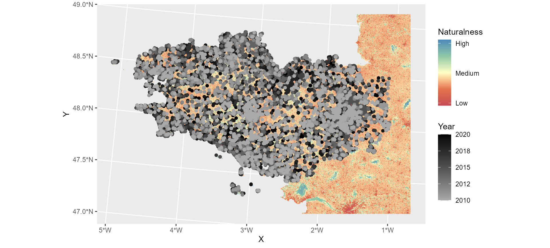
SSI calculation
The function was designed to calculate SSI automatically from a dataset (for a taxon, a territory and a period). Several raster resolutions can be evaluated in a row.
A null distribution is generated by randomly selecting sites within the species range. The effect of the studied gradient is measured by the effect size between the simulated and the observed species distributions, repeated n times. A synanthropy score (SSI) is assigned to each species based on the average difference between the null and observed distributions (from 1 to 10).
Here, we execute the function for 3 resolutions (100, 200, 250), with 500 simulations each. Each species must have been found in a minimum of 30 cells to be evaluated (threshold argument). If you are in interactive mode, you will be prompted to validate the species list detected in the dataset. Make sure that there are no typos or synonyms, as each species will be considered separately for the analyses.
ssi_test <- SynAnthrop::ssi(r = ras_brittany,
               resolution = 100,
               data = spOcc,
               sim = 1,
               threshold = 30)
[Chunk tested in interactive mode only] Four different Pelophylax species are found in the dataset. Species determination is delicate for this genus, so we abort this run and group them as “Pelophylax spp.” before running the function.
spOcc %<>% mutate(Species = recode(Species,
                                   "Pelophylax kl. esculentus" = "Pelophylax spp.",
                                   "Pelophylax lessonae" = "Pelophylax spp.",
                                   "Pelophylax ridibundus" = "Pelophylax spp."))

ssi_results <- SynAnthrop::ssi(r = ras_brittany,
                   resolution = c(100, 200, 250),
                   data = spOcc,
                   sim = 500,
                   threshold = 30)
## Species found in the dataset:
## Alytes obstetricans
## Bombina variegata
## Bufo spinosus
## Epidalea calamita
## Hyla arborea
## Hyla meridionalis
## Ichthyosaura alpestris
## Lissotriton helveticus
## Pelodytes punctatus
## Pelophylax spp.
## Rana dalmatina
## Rana temporaria
## Salamandra salamandra
## Triturus marmoratus
## 2026-04-21 20:08:27.157961 - Aggregate naturalness raster cells at resolution 100 .
## 2026-04-21 20:08:32.812425 1 observation(s) were eliminated because of missing naturalness values
## 2026-04-21 20:08:32.951439 At this resolution, the landscape is divided into 157 * 108 cells (total = 10801 cells).
## You chose to evaluate species present in more than 30 cells.
## Species that will be evaluated are:
## Alytes obstetricans
## Bufo spinosus
## Epidalea calamita
## Hyla arborea
## Ichthyosaura alpestris
## Lissotriton helveticus
## Pelodytes punctatus
## Pelophylax spp.
## Rana dalmatina
## Rana temporaria
## Salamandra salamandra
## Triturus marmoratus
##
## 2026-04-21 20:08:38.94487 - Generating null distributions for:
## 2026-04-21 20:08:38.945181 Alytes obstetricans (1/12)
## Simulation 1/500... 100/500... 200/500... 300/500... 400/500... 500/500
## 2026-04-21 20:08:51.759809 Bufo spinosus (2/12)
## Simulation 1/500... 100/500... 200/500... 300/500... 400/500... 500/500
## 2026-04-21 20:10:23.028778 Epidalea calamita (3/12)
## Simulation 1/500... 100/500... 200/500... 300/500... 400/500... 500/500
## 2026-04-21 20:10:32.414624 Hyla arborea (4/12)
## Simulation 1/500... 100/500... 200/500... 300/500... 400/500... 500/500
## 2026-04-21 20:10:55.455802 Ichthyosaura alpestris (5/12)
## Simulation 1/500... 100/500... 200/500... 300/500... 400/500... 500/500
## 2026-04-21 20:11:06.732096 Lissotriton helveticus (6/12)
## Simulation 1/500... 100/500... 200/500... 300/500... 400/500... 500/500
## 2026-04-21 20:11:55.559296 Pelodytes punctatus (7/12)
## Simulation 1/500... 100/500... 200/500... 300/500... 400/500... 500/500
## 2026-04-21 20:12:04.800416 Pelophylax spp. (8/12)
## Simulation 1/500... 100/500... 200/500... 300/500... 400/500... 500/500
## 2026-04-21 20:12:42.863752 Rana dalmatina (9/12)
## Simulation 1/500... 100/500... 200/500... 300/500... 400/500... 500/500
## 2026-04-21 20:13:17.747012 Rana temporaria (10/12)
## Simulation 1/500... 100/500... 200/500... 300/500... 400/500... 500/500
## 2026-04-21 20:13:51.335355 Salamandra salamandra (11/12)
## Simulation 1/500... 100/500... 200/500... 300/500... 400/500... 500/500
## 2026-04-21 20:14:43.518382 Triturus marmoratus (12/12)
## Simulation 1/500... 100/500... 200/500... 300/500... 400/500... 500/500
##
## 2026-04-21 20:15:05.280103 - Calculating effect sizes...
## Simulation 1/500... 100/500... 200/500... 300/500... 400/500... 500/500
## 2026-04-21 20:23:44.946399 Analysis finished for resolution 100
## 2026-04-21 20:23:44.950471 - Aggregate naturalness raster cells at resolution 200 .
## 2026-04-21 20:23:51.723144 0 observation(s) were eliminated because of missing naturalness values
## 2026-04-21 20:23:51.866775 At this resolution, the landscape is divided into 79 * 54 cells (total = 2780 cells).
## You chose to evaluate species present in more than 30 cells.
## Species that will be evaluated are:
## Alytes obstetricans
## Bufo spinosus
## Epidalea calamita
## Hyla arborea
## Ichthyosaura alpestris
## Lissotriton helveticus
## Pelodytes punctatus
## Pelophylax spp.
## Rana dalmatina
## Rana temporaria
## Salamandra salamandra
## Triturus marmoratus
##
## 2026-04-21 20:23:57.187772 - Generating null distributions for:
## 2026-04-21 20:23:57.188095 Alytes obstetricans (1/12)
## Simulation 1/500... 100/500... 200/500... 300/500... 400/500... 500/500
## 2026-04-21 20:24:06.235306 Bufo spinosus (2/12)
## Simulation 1/500... 100/500... 200/500... 300/500... 400/500... 500/500
## 2026-04-21 20:24:34.756606 Epidalea calamita (3/12)
## Simulation 1/500... 100/500... 200/500... 300/500... 400/500... 500/500
## 2026-04-21 20:24:41.118194 Hyla arborea (4/12)
## Simulation 1/500... 100/500... 200/500... 300/500... 400/500... 500/500
## 2026-04-21 20:24:54.661984 Ichthyosaura alpestris (5/12)
## Simulation 1/500... 100/500... 200/500... 300/500... 400/500... 500/500
## 2026-04-21 20:25:02.541803 Lissotriton helveticus (6/12)
## Simulation 1/500... 100/500... 200/500... 300/500... 400/500... 500/500
## 2026-04-21 20:25:24.875237 Pelodytes punctatus (7/12)
## Simulation 1/500... 100/500... 200/500... 300/500... 400/500... 500/500
## 2026-04-21 20:25:30.885451 Pelophylax spp. (8/12)
## Simulation 1/500... 100/500... 200/500... 300/500... 400/500... 500/500
## 2026-04-21 20:25:51.058967 Rana dalmatina (9/12)
## Simulation 1/500... 100/500... 200/500... 300/500... 400/500... 500/500
## 2026-04-21 20:26:09.568292 Rana temporaria (10/12)
## Simulation 1/500... 100/500... 200/500... 300/500... 400/500... 500/500
## 2026-04-21 20:26:27.110393 Salamandra salamandra (11/12)
## Simulation 1/500... 100/500... 200/500... 300/500... 400/500... 500/500
## 2026-04-21 20:26:55.338329 Triturus marmoratus (12/12)
## Simulation 1/500... 100/500... 200/500... 300/500... 400/500... 500/500
##
## 2026-04-21 20:27:11.444616 - Calculating effect sizes...
## Simulation 1/500... 100/500... 200/500... 300/500... 400/500... 500/500
## 2026-04-21 20:34:59.403469 Analysis finished for resolution 200
## 2026-04-21 20:34:59.415998 - Aggregate naturalness raster cells at resolution 250 .
## 2026-04-21 20:35:06.375382 1 observation(s) were eliminated because of missing naturalness values
## 2026-04-21 20:35:06.527229 At this resolution, the landscape is divided into 65 * 44 cells (total = 1837 cells).
## You chose to evaluate species present in more than 30 cells.
## Species that will be evaluated are:
## Alytes obstetricans
## Bufo spinosus
## Epidalea calamita
## Hyla arborea
## Ichthyosaura alpestris
## Lissotriton helveticus
## Pelodytes punctatus
## Pelophylax spp.
## Rana dalmatina
## Rana temporaria
## Salamandra salamandra
## Triturus marmoratus
##
## 2026-04-21 20:35:09.730361 - Generating null distributions for:
## 2026-04-21 20:35:09.730705 Alytes obstetricans (1/12)
## Simulation 1/500... 100/500... 200/500... 300/500... 400/500... 500/500
## 2026-04-21 20:35:19.260519 Bufo spinosus (2/12)
## Simulation 1/500... 100/500... 200/500... 300/500... 400/500... 500/500
## 2026-04-21 20:35:49.554813 Epidalea calamita (3/12)
## Simulation 1/500... 100/500... 200/500... 300/500... 400/500... 500/500
## 2026-04-21 20:35:57.085975 Hyla arborea (4/12)
## Simulation 1/500... 100/500... 200/500... 300/500... 400/500... 500/500
## 2026-04-21 20:36:15.110536 Ichthyosaura alpestris (5/12)
## Simulation 1/500... 100/500... 200/500... 300/500... 400/500... 500/500
## 2026-04-21 20:36:24.273629 Lissotriton helveticus (6/12)
## Simulation 1/500... 100/500... 200/500... 300/500... 400/500... 500/500
## 2026-04-21 20:36:43.259223 Pelodytes punctatus (7/12)
## Simulation 1/500... 100/500... 200/500... 300/500... 400/500... 500/500
## 2026-04-21 20:36:50.020429 Pelophylax spp. (8/12)
## Simulation 1/500... 100/500... 200/500... 300/500... 400/500... 500/500
## 2026-04-21 20:37:11.170849 Rana dalmatina (9/12)
## Simulation 1/500... 100/500... 200/500... 300/500... 400/500... 500/500
## 2026-04-21 20:37:31.809184 Rana temporaria (10/12)
## Simulation 1/500... 100/500... 200/500... 300/500... 400/500... 500/500
## 2026-04-21 20:37:48.820151 Salamandra salamandra (11/12)
## Simulation 1/500... 100/500... 200/500... 300/500... 400/500... 500/500
## 2026-04-21 20:38:13.947375 Triturus marmoratus (12/12)
## Simulation 1/500... 100/500... 200/500... 300/500... 400/500... 500/500
##
## 2026-04-21 20:38:26.810032 - Calculating effect sizes...
## Simulation 1/500... 100/500... 200/500... 300/500... 400/500... 500/500
## 2026-04-21 20:46:32.330981 Analysis finished for resolution 250
## 2026-04-21 20:46:32.362803 Analysis completed.Visualise and analyse the SSI results
The SSI function produces 3 data frames.
SSI and effect sizes per species
The first table contains the SSI calculated per species and resolution. It is a summary table containing one line per species per resolution, with the mean effect size, the number of simulations, and the SSI Index (1 to 10).
head(sp_ssi <- ssi_results$speciesScores)## # A tibble: 6 × 5
## Species mean nRun Index Resolution
## <chr> <dbl> <int> <dbl> <dbl>
## 1 Alytes obstetricans 0.0293 500 2 100
## 2 Bufo spinosus 0.0578 500 2 100
## 3 Epidalea calamita -0.447 500 10 100
## 4 Hyla arborea 0.00389 500 3 100
## 5 Ichthyosaura alpestris -0.0584 500 4 100
## 6 Lissotriton helveticus -0.108 500 4 100The second table is a data.frame compiling the effect sizes (effsize)
calculated for each comparison of simulated (Null) and observed data,
for each species and resolution. The sample sizes for simulated (n1) and
observed (n2) data are specified, as well as the magnitude of the effect
size (negligible < small < moderate < large) provided by
rstatix::cohens_d.
head(effsize_res <- ssi_results$effSizes)## # A tibble: 6 × 10
## .y. group1 group2 effsize n1 n2 magnitude Species Run Resolution
## <chr> <chr> <chr> <dbl> <int> <int> <ord> <chr> <int> <dbl>
## 1 value Null Observed -0.349 391 391 small Trituru… 1 100
## 2 value Null Observed -0.0107 1705 1705 negligible Salaman… 1 100
## 3 value Null Observed -0.196 949 949 negligible Rana te… 1 100
## 4 value Null Observed -0.0424 1028 1028 negligible Rana da… 1 100
## 5 value Null Observed 0.108 1156 1156 negligible Pelophy… 1 100
## 6 value Null Observed -0.373 121 121 small Pelodyt… 1 100Here we combine these two tables to visualize effect sizes and SSI obtained with the resolution 100.
# keep only data for resolution 100
# associate the SSI to the detailed effect sizes
sub_effsize_res <- effsize_res %>%
  filter(Resolution == 100) %>%
  left_join(sp_ssi, by = c("Species", "Resolution"))

# make the score a factor
sub_effsize_res$Index <- as.factor(sub_effsize_res$Index)

# plot the results
ggplot(sub_effsize_res,
       aes(x = reorder(Species, -effsize),
           y = -effsize, fill = Index)) +
  geom_hline(yintercept = 0.0, color = "darkgrey",
             linewidth = 0.8, linetype = "dashed") +
  geom_boxplot() +
  coord_flip() +
  scale_fill_brewer(name = "SSI", palette = "RdYlGn") +
  ylab("Effect size") +
  xlab("Species") +
  theme(axis.title.y = element_blank()) +
  theme(legend.position.inside = c(0.9, 0.2)) +
  theme_bw()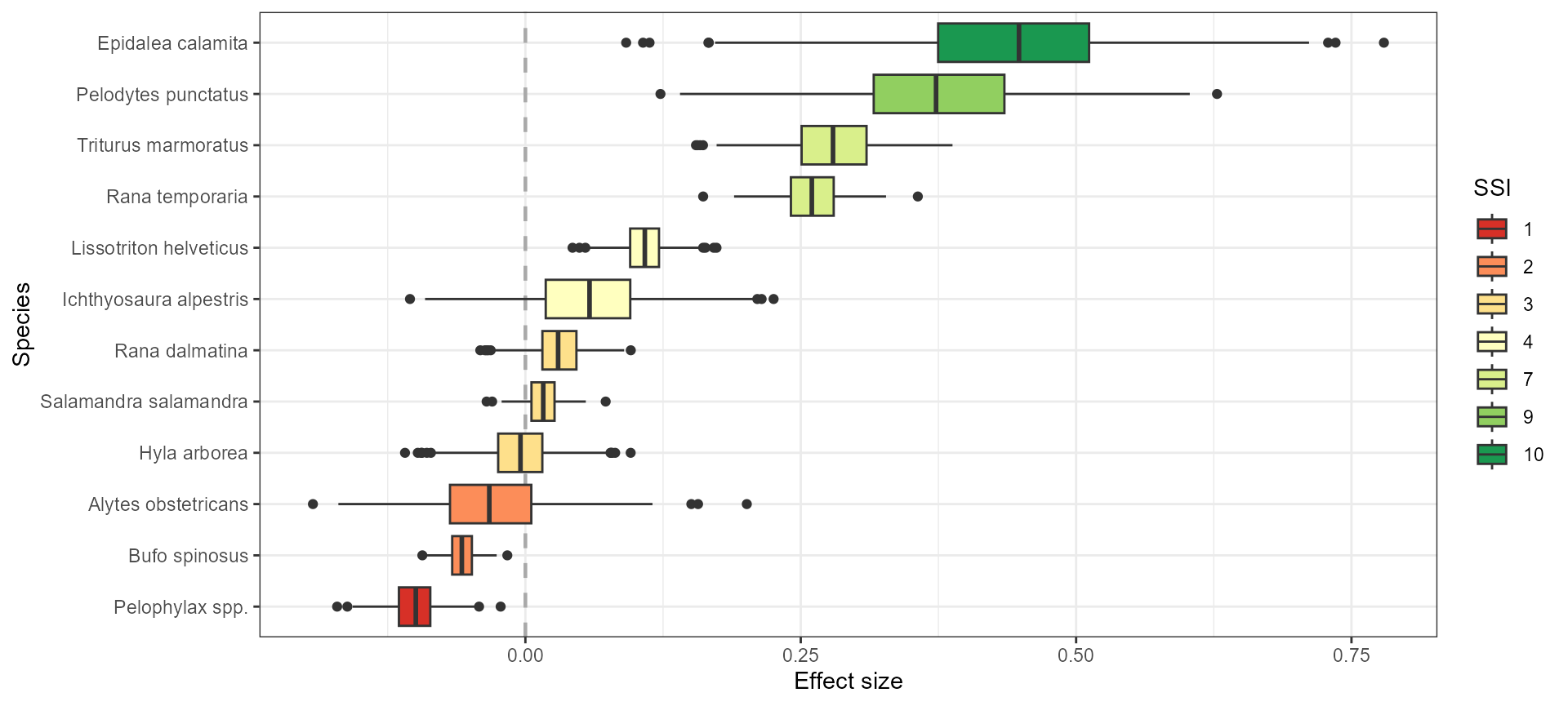
Based on this plot, we observe that species have contrasted SSI. Epidalea calamita shows high affinity for anthropogenic systems (SSI = 10), followed by Pelodytes punctatus, Triturus marmoratus, and Rana temporaria that all have positive effect sizes. On the opposite end of the gradient, green frogs (Pelophylax spp. and Pelophylax kl. esculentus) have low synanthropy scores (SSI = 1), and negative effect sizes along with Bufo spinosus.
Resolution comparison
It is useful to check whether scores are affected by the level of data aggregation operated during the process. We create a graph that allows the comparison of scores and species ranks across data resolutions.
# change resolution class
sp_ssi$Resolution <- as.factor(sp_ssi$Resolution)

CGPfunctions::newggslopegraph(dataframe = sp_ssi,
                Resolution,
                Index,
                Grouping = Species,
                Title = "Synanthropy scores for amphibian species in western France",
                SubTitle = NULL,
                Caption = NULL)
##
## Converting 'Resolution' to an ordered factor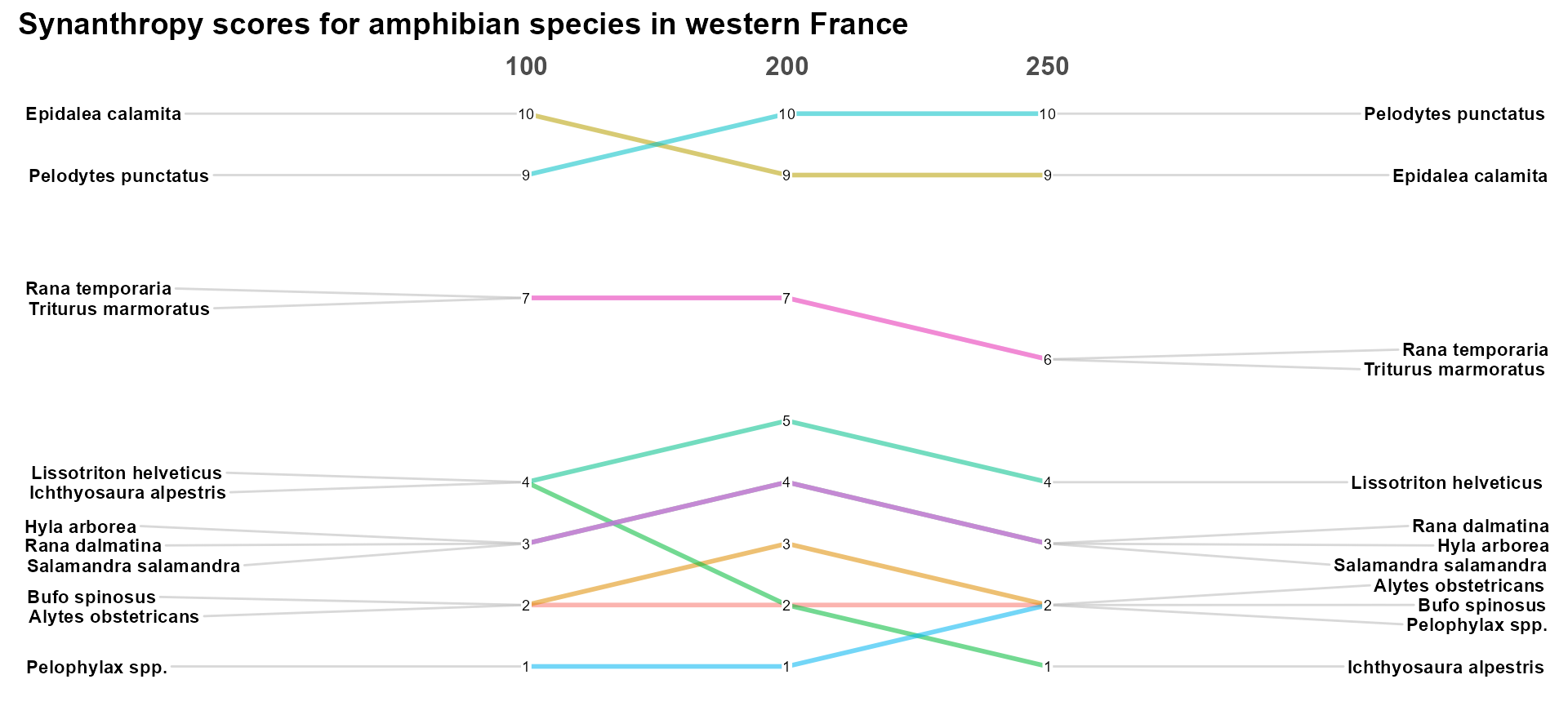
Interestingly, scores are not affected much by the change in data resolution, with unchanged ranks for species with SSI > 4. This suggests that the evaluation is robust to data aggregation.
Distribution map
Finally, the third table contains all the points simulated and observed.
head(points <- ssi_results$samplesList)## cell simulation Species variable x y Resolution
## 1 7736 1 Triturus marmoratus Null 342207.6 6805184 100
## 2 8033 1 Triturus marmoratus Null 288207.6 6801184 100
## 3 9522 1 Triturus marmoratus Null 350207.6 6783184 100
## 4 6765 1 Triturus marmoratus Null 344207.6 6817184 100
## 5 8494 1 Triturus marmoratus Null 238207.6 6795184 100
## 6 2634 1 Triturus marmoratus Null 182207.6 6867184 100We can visualize the locations of observations and of one set of randomly selected sites for each species.
# we select one resolution, one set of simulated points, and the observed points
sub_points <- points %>% filter(Resolution == "100",
                                simulation %in% c(1, "no"))

ggplot() +
  geom_point(data = sub_points, aes(x = x, y = y, color = variable),
             size = 1.5, alpha = 0.5) +
  scale_color_manual(values = c("#ff6600", "#660099")) +
  theme(axis.title.x = element_blank(),
        axis.title.y = element_blank()) +
  guides(color = guide_legend(title = "Points")) +
  facet_wrap(. ~ Species) +
  theme_void()
## Warning: Removed 603 rows containing missing values or values outside the scale range
## (`geom_point()`).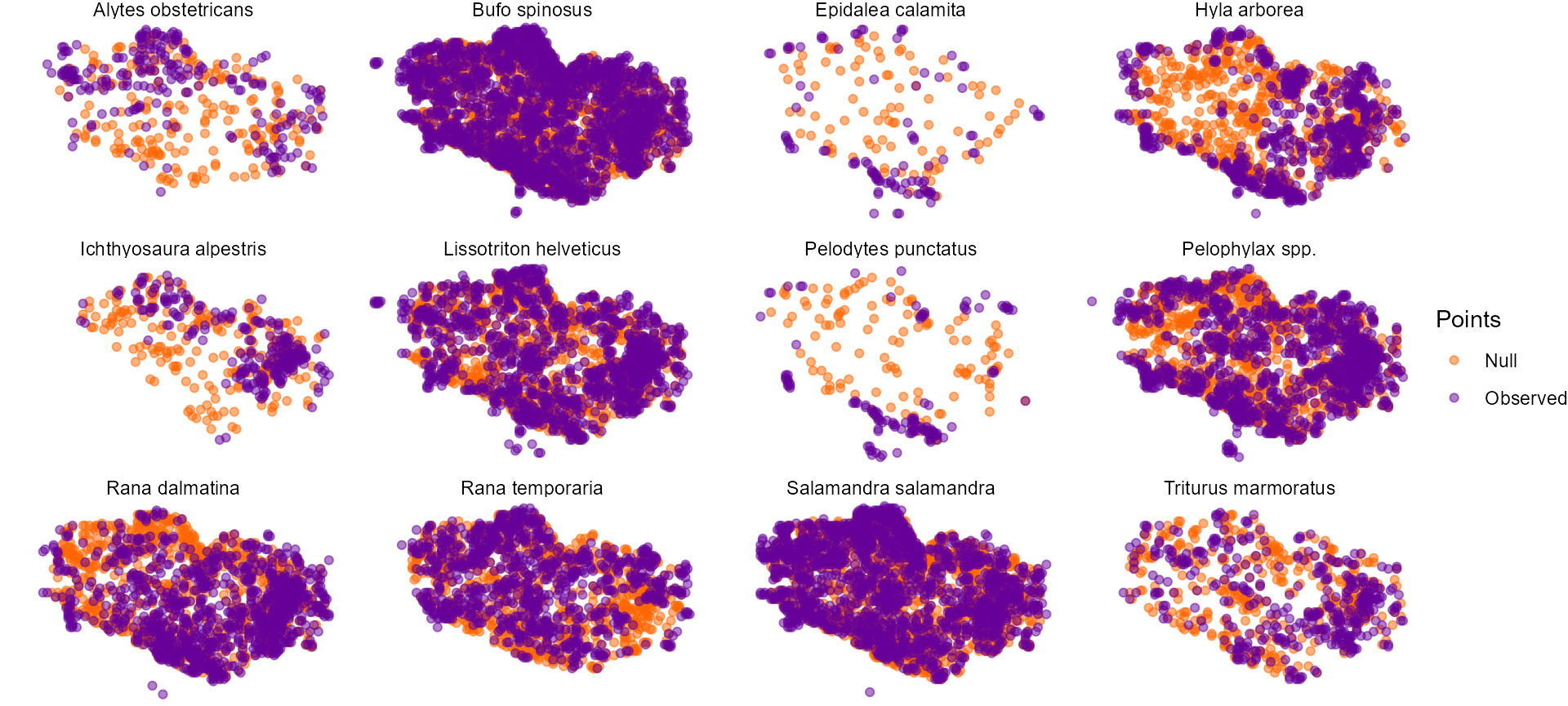
2- Synanthropy Community Score: application of the SSI to amphibian communities in ponds
The scores may then be used at the community scale to estimate the overall sensitivity of assemblages to land use change. These average scores are complementary to anthropisation maps, which must be considered as potential. Indeed, there are cases where the maps present values higher than the scores when sensitive species are not detected, and cases where the maps present values lower than the scores when in reality some populations of sensitive species have maintained themselves locally.
Here we test the scores obtained in the previous section with data of amphibian communities surveyed in western France (around the city of Rennes) between 2000 and 2010.
Setup
We load the dataset and take a look at it. Its structure is similar to that of the previous dataset, with columns for species names, year, and site of sampling, abundance, and XY coordinates.
ex_com <- read.table(file.path(here::here(), "data",
                               "amphibiansBrittany",
                               "Amphibian_community_MNIE.csv"), sep=";", h=T)
head(ex_com)
## Species X Y Abundance Years Site
## 1 Bufo spinosus 357337 6783846 1 2010 Site 136
## 2 Pelodytes punctatus 348398 6785920 1 2010 Site 58
## 3 Rana dalmatina 357337 6783846 1 2010 Site 136
## 4 Salamandra salamandra 357337 6783846 1 2010 Site 136
## 5 Hyla arborea 344270 6809372 1 2009 Site 29
## 6 Ichthyosaura alpestris 353382 6782286 1 2006 Site 109Because not all species were attributed a SSI based on the threshold number applied, we need to check whether some species will not have a SSI in this community.
# species that are in the community dataset, that are not in the SSI dataset
sub_sp_ssi <- sp_ssi %>% filter(Resolution == "100")
(unevaluated_species <- setdiff(unique(ex_com$Species), unique(sub_sp_ssi$Species)))
## [1] "Triturus cristatus" "Lissotriton vulgaris" "Pelophylax lessonae"
# total number of sites sampled
nsites <- ex_com %>% count(Site) %>% nrow()

# proportion of communities these species are present in
ex_com %>%
  filter(Species %in% unevaluated_species) %>%
  count(Site) %>%
  nrow()/ nsites
## [1] 0.34636873 species of the community dataset do not have a SSI and they are present in 34% of the studied communities. Community analyses must be interpreted with this caveat in mind.
We then associate previously calculated SSI at resolution 100 to each species, and calculate for each site the species richness, SCS, i.e. the mean of SSI, and SCS, i.e. the SCS weighted by species abundance.
ex_com_evaluated <- ex_com %>% inner_join(sub_sp_ssi %>% select(Species, Index))## Joining with `by = join_by(Species)`
head(ex_com_sites <- ex_com_evaluated %>%
  group_by(Site, Years, X, Y) %>%
  summarise(Richness = n_distinct(Species),
            SCS = round(mean(Index), 2),
            SCSw = round(weighted.mean(Index, Abundance), 2)))
## `summarise()` has grouped output by 'Site', 'Years', 'X'. You can override
## using the `.groups` argument.## # A tibble: 6 × 7
## # Groups: Site, Years, X [6]
## Site Years X Y Richness SCS SCSw
## <chr> <int> <int> <int> <int> <dbl> <dbl>
## 1 Site 1 2010 335076 6788565 3 3.33 3.2
## 2 Site 10 2010 340610 6790480 5 3.8 3.8
## 3 Site 100 2010 351549 6778613 5 3.8 3.89
## 4 Site 101 2010 351550 6778573 3 3.67 3.67
## 5 Site 102 2010 351577 6780908 3 2.67 3.54
## 6 Site 103 2010 351641 6778430 4 2.75 3.74We also calculated the Synanthropy Community Index (SCI), an equivalent of the Floristic Quality Index to account for variation of species richness, using the following formula :
\[ SCI = SCS(√ richness) \]
ex_com_sites %<>% mutate(SCI = round(SCS * sqrt(Richness), 2),
                        SCIw = round(SCSw * sqrt(Richness), 2))

head(ex_com_sites)
## # A tibble: 6 × 9
## # Groups: Site, Years, X [6]
## Site Years X Y Richness SCS SCSw SCI SCIw
## <chr> <int> <int> <int> <int> <dbl> <dbl> <dbl> <dbl>
## 1 Site 1 2010 335076 6788565 3 3.33 3.2 5.77 5.54
## 2 Site 10 2010 340610 6790480 5 3.8 3.8 8.5 8.5
## 3 Site 100 2010 351549 6778613 5 3.8 3.89 8.5 8.7
## 4 Site 101 2010 351550 6778573 3 3.67 3.67 6.36 6.36
## 5 Site 102 2010 351577 6780908 3 2.67 3.54 4.62 6.13
## 6 Site 103 2010 351641 6778430 4 2.75 3.74 5.5 7.48Map the results
We can now visualize our new index.
# Create spatial objects
ex_com_map <- sf::st_as_sf(ex_com_sites, coords = c("X", "Y"), crs = 2154)
ras_com <- raster::crop(ras_brittany, ex_com_map)

# Plot the map
ggplot() +
  tidyterra::geom_spatraster(data = ras_com, alpha = 0.8) +
  geom_sf(data = ex_com_map, aes(color = SCIw, size = Richness)) +
  scale_colour_gradient(low = "yellow", high = "darkgreen") +
  tidyterra::scale_fill_whitebox_c(palette = "muted", direction=-1) +
  ggtitle("Amphibian communities in ponds") +
  theme(legend.position = "bottom")
## <SpatRaster> resampled to 501102 cells.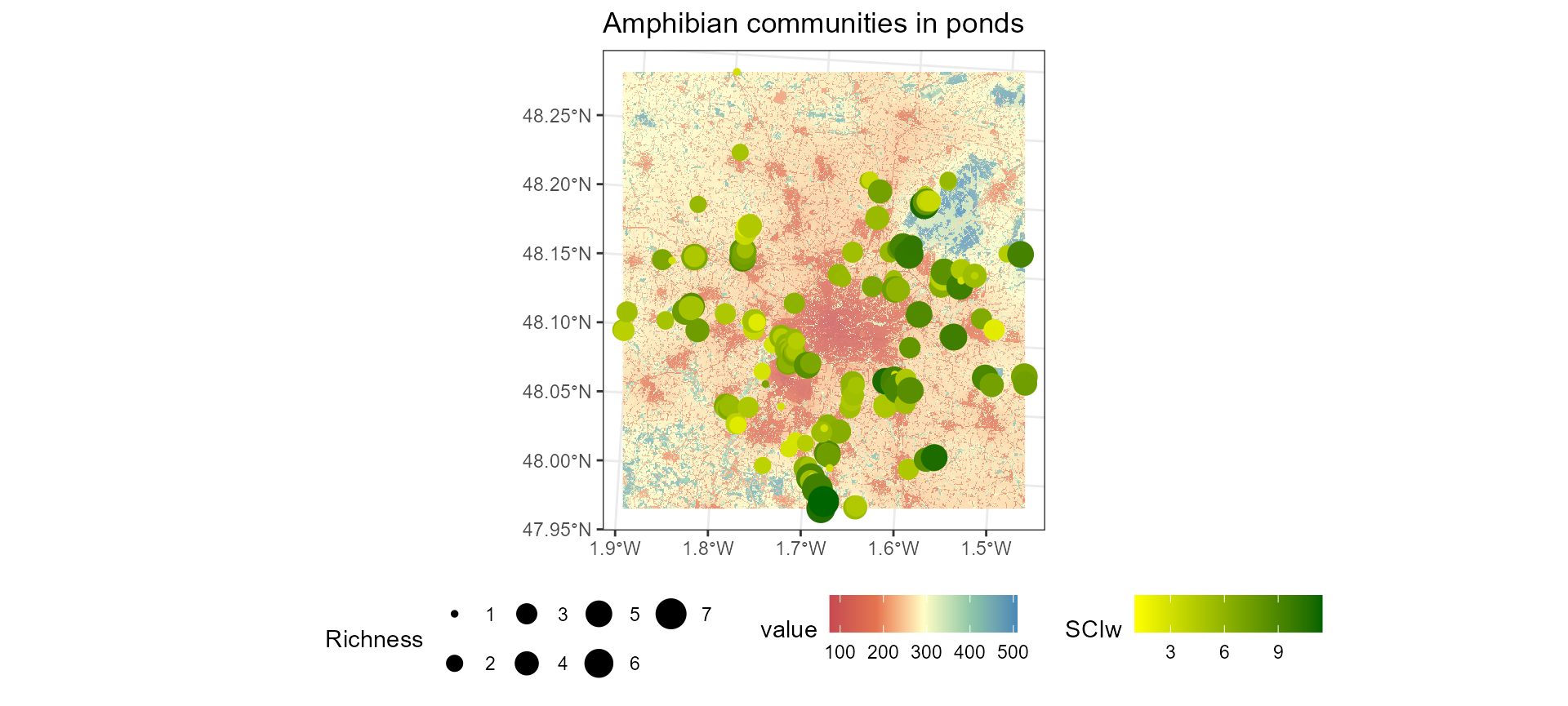
On this map, the background shows the naturalness index with lower (red) values indicating low naturalness and higher (blue) values indicating high naturalness. Point size represents the amphibian community richness. Lighter green points identify the ponds that have less synanthropic assemblages and are therefore potentially more sensitive to urbanisation and intensified land-use. Darker green points distinguish the ponds presenting rather synanthropic assemblages. It is interesting to note that these results contrast in part with the map, with some examples of communities with low SCI scores in areas with low naturalness, illustrating the complementarity of the two approaches.
Citations
Citations: * Morel L. 2023. SynAnthrop: Species distribution and sensitivity to anthropisation, R package version 0.1.1, https://github.com/lomorel/SynAnthrop
UMR DECOD, lois.morel@institut-agro.fr↩︎
UMR EcoBio, nadege.belouard@gmail.com↩︎